Option Pricing Models

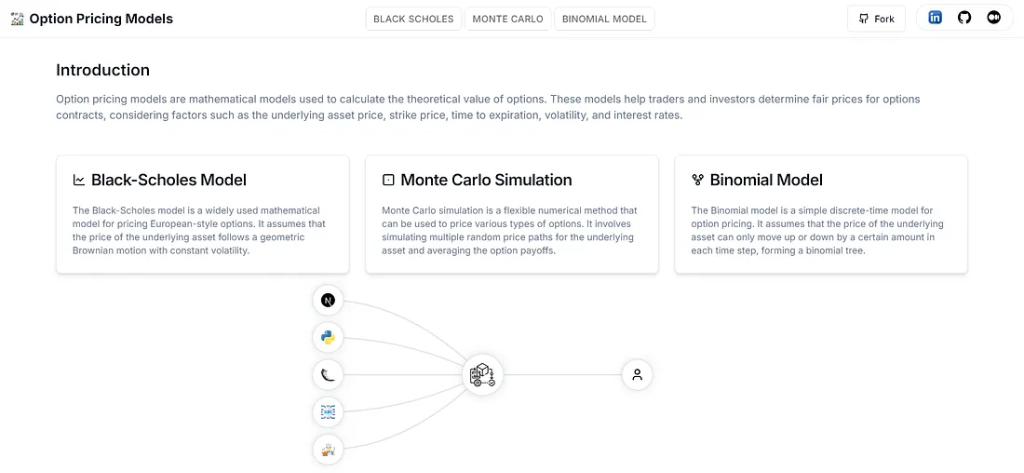
Options are among the most versatile financial instruments available today, offering traders the ability to hedge exposure, speculate on direction, and manage risk across a spectrum of market conditions. Accurate option pricing is crucial, not just for direct execution, but for delta hedging, portfolio optimization, and multi-asset risk management. This article breaks down the mathematical foundations and provides standard implementations for the three cornerstones of quantitative options pricing: the Black-Scholes model, Monte Carlo simulation, and the Binomial tree method.

An option contract gives the buyer the right, but not the obligation, to buy (a Call) or sell (a Put) an underlying asset at a strike price K before or at an expiration date T. The theoretical value of an option is governed by five primary inputs: the spot price of the underlying asset (S), the strike price (K), the time to maturity (T), the risk-free interest rate (r), and the asset's annualized volatility (σ).

To understand how these inputs interact, quant developers and risk managers use three distinct mathematical approaches to price contracts: continuous analytical solutions, stochastic simulations, and discrete time-stepping trees.

Introduced in 1973 by Fischer Black, Myron Scholes, and Robert Merton, the Black-Scholes model is the foundational framework of modern quantitative finance. It provides a closed-form analytical solution for European call and put options (which can only be exercised at maturity).

The model operates under strict theoretical assumptions: the underlying asset price follows a Geometric Brownian Motion (GBM) with constant volatility σ and drift r, there are no transaction costs or dividends, and borrowing/lending can occur continuously at the risk-free rate.

Here is the standard implementation of the Black-Scholes pricing formula for Call and Put options using Python's scipy.stats.norm distribution helper:

# Black-Scholes European call/put option pricing model
import numpy as np
from scipy.stats import norm

def black_scholes(S, K, T, r, sigma, option_type="call"):
    # Calculate d1 and d2 components
    d1 = (np.log(S / K) + (r + 0.5 * sigma**2) * T) / (sigma * np.sqrt(T))
    d2 = d1 - sigma * np.sqrt(T)
    
    if option_type.lower() == "call":
        # Call Payoff = S * N(d1) - K * e^(-rT) * N(d2)
        return S * norm.cdf(d1) - K * np.exp(-r * T) * norm.cdf(d2)
    elif option_type.lower() == "put":
        # Put Payoff = K * e^(-rT) * N(-d2) - S * N(-d1)
        return K * np.exp(-r * T) * norm.cdf(-d2) - S * norm.cdf(-d1)
    else:
        raise ValueError("Option type must be 'call' or 'put'")

While Black-Scholes is computationally instantaneous, its assumption of constant volatility leads to the famous 'volatility smile' in real-world markets, where out-of-the-money options trade at higher implied volatilities than those at-the-money.

For complex or path-dependent derivatives (like Asian average-rate options or barrier options), analytical solutions are often mathematically impossible. Here, we turn to Monte Carlo simulation. Instead of solving a differential equation, we simulate thousands of possible future price paths for the underlying asset, calculate the option's payoff on each path, discount those payoffs to the present, and average them.

The underlying asset price path is modeled as a stochastic process using Geometric Brownian Motion (GBM):

` S_T = S_0 exp( (r - 0.5 σ^2)T + σ sqrt(T) * Z ) ` Where Z is a random variable drawn from a standard normal distribution.

Here is a vector-optimized NumPy implementation of Monte Carlo pricing for European call and put options:

# Monte Carlo simulation for European option pricing
import numpy as np

def monte_carlo_pricing(S, K, T, r, sigma, num_simulations=100000, option_type="call"):
    # Generate random standard normal variables
    Z = np.random.standard_normal(num_simulations)
    
    # Simulate terminal stock prices using Geometric Brownian Motion
    ST = S * np.exp((r - 0.5 * sigma**2) * T + sigma * np.sqrt(T) * Z)
    
    # Calculate raw option payoffs at maturity
    if option_type.lower() == "call":
        payoffs = np.maximum(ST - K, 0)
    elif option_type.lower() == "put":
        payoffs = np.maximum(K - ST, 0)
    else:
        raise ValueError("Option type must be 'call' or 'put'")
        
    # Discount payoffs back to present value and take the expectation
    option_price = np.exp(-r * T) * np.mean(payoffs)
    return option_price

The key advantage of Monte Carlo simulation is its extreme flexibility, as it can accommodate any path dependency or complex barrier condition. Its downside is computational overhead: to achieve high precision, you must run millions of paths, which requires optimized parallel code or hardware acceleration.

Introduced by Cox, Ross, and Rubinstein in 1979, the Binomial Tree method is a discrete-time model. It represents the future asset price as a recombining tree, where at each time step dt, the price can either scale up by factor u or down by factor d.

S0 * u * u
                       /
                S0 * u ── 
               /       \
        S0 ── ──        S0 * u * d
               \       /
                S0 * d ── 
                       \
                        S0 * d * d

Unlike Black-Scholes, the Binomial Tree method can price American options. Because American options can be exercised early (before maturity T), the pricing algorithm works backward from the terminal nodes, comparing the intrinsic payoff of early exercise against the discounted continuation value at every node.

Here is a dynamic programming implementation of the Cox-Ross-Rubinstein Binomial Tree for European and American options:

# Binomial Tree pricing model supporting American options
import numpy as np

def binomial_tree_pricing(S, K, T, r, sigma, N=100, option_type="call", american=True):
    dt = T / N
    # Calculate up, down, and risk-neutral probability parameters
    u = np.exp(sigma * np.sqrt(dt))
    d = 1 / u
    p = (np.exp(r * dt) - d) / (u - d)
    
    # Generate stock prices at maturity nodes
    S_tree = S * (u ** np.arange(N, -1, -1)) * (d ** np.arange(0, N + 1))
    
    # Initialize option values at expiration
    if option_type.lower() == "call":
        V = np.maximum(S_tree - K, 0)
    elif option_type.lower() == "put":
        V = np.maximum(K - S_tree, 0)
    else:
        raise ValueError("Option type must be 'call' or 'put'")
        
    # Step backward through the tree to calculate present values
    for i in range(N - 1, -1, -1):
        continuation = np.exp(-r * dt) * (p * V[:-1] + (1 - p) * V[1:])
        
        if american:
            # Fetch spot prices at current time step nodes
            S_node = S * (u ** np.arange(i, -1, -1)) * (d ** np.arange(0, i + 1))
            intrinsic = np.maximum(S_node - K, 0) if option_type.lower() == "call" else np.maximum(K - S_node, 0)
            # Take maximum of early exercise vs holding
            V = np.maximum(intrinsic, continuation)
        else:
            V = continuation
            
    return V[0]

Beyond basic valuation, managing options risk requires understanding their sensitivities to changing market conditions. These sensitivities are measured by the Greeks, which are partial derivatives of the pricing formula:

• Delta (Δ): Sensitivity of the option price to small changes in the underlying spot price.

• Gamma (Γ): Acceleration of Delta, which is the sensitivity of Delta to changes in the spot price.

• Theta (Θ): Sensitivity of the option price to the decay of time to maturity.

• Vega (ν): Sensitivity of the option price to changes in implied volatility.

• Rho (ρ): Sensitivity of the option price to interest rate changes.

OptionLab leverages heatmaps to visualize these sensitivities, allowing traders to see how the option's value moves across a 2D coordinate space of spot prices and implied volatilities.

Option pricing is a fundamental core of quantitative finance. By combining analytic closed-forms (Black-Scholes), stochastic projections (Monte Carlo), and discrete lattices (Binomial Tree), quants can evaluate and hedge risk for even the most complex derivatives.

To explore the interactive dashboard yourself, visit OptionLab. You can also view the complete source code and mathematical libraries on GitHub: https://github.com/shaikhmubin02/option-pricing-models.git.